Simantics System Dynamics
Contents
What is Simantics System Dynamics
Simantics System Dynamics is currently the only open source modelling and simulating tool for Simantics. Simantics System Dynamics is under development and will go through changes in the future. New features will be added and old ones improved according to the needs of modellers.
This documentation introduces you to the current version of Simantics System Dynamics. The documentation includes basic modelling principles and a guide on how to model system dynamics models with Simantics System Dynamics. If you like to get to know the tool better and try modelling and simulating yourself, install the software and try our basic and advanced tutorials!
Introduction to System Dynamics Simulation
System Dynamics
System dynamics is an approach to understanding different organizations, markets and other complex systems and their dynamic behavior. Simantics System Dynamics is a free modelling tool for system dynamics modeling and simulation. See installation instructions.
Model
System dynamics model is generally understood as the model configuration. In this tool, the model contains also other components: Experiments are the way to simulate the model. You can have experiments with different configurations, for example different initial values for some parameters. In that way, you don't have to always configure the model for different scenarios. Module types allow user to create reusable component types which can be instantiated as Modules. The Modules folder contains all the different module types in your model and you can create new module types there. The Functions folder contains built-in and user-defined functions.
Model structure
Components
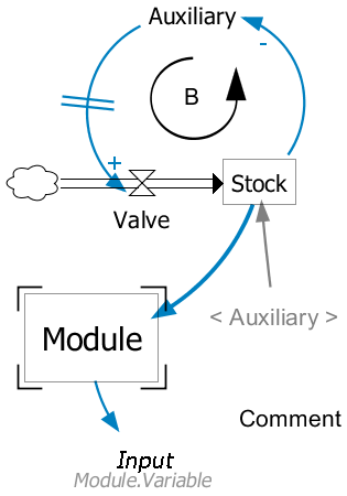
Most of the components you can use in your models are basic system dynamics components. The modularity of the models introduces two additional components, Modules and Inputs. All the components are explained below.
Component types
Auxiliary
Auxiliary is the most basic variable you can use. It represents a single value or a mathematical expression. There are different types of auxiliary variables currently in the system: Auxiliary, Parameter, Constant, Delay and WithLookup. Auxiliary is the default type. Parameters are static values that the user can change. When only parameters are changed, the model simulates faster, because the system does not have to recompile the model. WithLookup and Delay are special variables. WithLookup has an expression and a lookup table. The expression defines what value is taken from the defined table. Delay variable delays an equation a given time with a given delay order.
Dependency
Dependency is an arrow that connects two components. It means that the value of the variable from which the arrow starts is used to calculate the value of the variable where the arrow ends. Dependencies that are used for a stock initial value only are colored grey by default, in contrast to the regular blue dependency arrows.
Flow
Flow connects clouds, valves and stocks. Flow represents an actual flow of something from stocks or clouds to stocks or clouds. There has to be at least one valve in a flow and the system creates it automatically, if none of the ends of the flow is a valve.
Valve
Valve regulates the rate of a flow. The value of a valve is automatically used in calculating the level of an adjacent stock. Valves behave just like Auxiliary variables but look different and you can connect also flows to them.
Stock
The value of a stock variable is an integral of flows leaving and flows arriving to the variable. The integral is calculated automatically from the valves that are connected to the variable with flow connections. Alternatively, the equation that is integrated can be defined manually by user. A stock must be given an initial value. Initial value can be a single value or an equation. You can use values of other variables to calculate the initial value.
Cloud
Cloud is not a variable. It represents a starting or ending point of a flow, if it is not in the scope of the model.
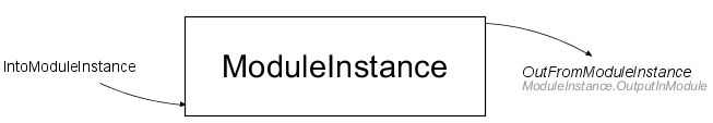
Module
Modules enable structural modeling. Modules are defined just like the basic model configuration, but the module component hides the actual configuration. You can only connect dependency connections into the module and dependency connections from the module must end to Input variables. The interface of the module is defined using input and output variables in the configuration of the module. All variable types can be set as output variables. If a variable is an output variable, its font is bold.
Input
Input variables are the way of getting values from other modules. Inputs look like auxiliary variables except their font is italics. You can set a default value to the input variable in case it is not connected to any variable. Connections are made from the modules properties, when the module is populated. Input doesn't have to be connected with an arrow to a module. If the variable has no connections, it can get values from a higher level in the hierarchy. If an input is connected to an output, the output and its module are shown below the variable using dot notation.
Shadow
Shadow variable is a reference to a variable defined elsewhere on the diagram. The referred variable can be an auxiliary, a valve, a stock, or an input. Dependency and flow arrows can be drawn out of a shadow variable, but no arrows can be drawn into a shadow variable. Shadow variables are used to improve the readability of the model.
Loop
Loop element is a graphical component for highlighting selected feedback loops in a model.
Comment
Comment element is a string of text on diagram.
Modeling Principles
System dynamics modelling is much more than just mathematical formulas and nice graphs. Models are ways of communicating. There are some basic principles in system dynamics modelling that make the models easier to read and understand. You do not have to apply these principles to simulate models, but using them makes it easier for you to communicate your model to others.
Variable names
Variables names should be nouns, not verbs. The names should be positive: for example it is easier to understand that satisfaction decreases than dissatisfaction rises. Variable names can and should have multiple words, if they are needed. Note that due to the reserved words in Modelica, variable names such as Carbon in Atmosphere cannot be used (in is a reserved word). Capitalizing the reserved (in → In) word can be used to sidestep the problem.
Connections
You should usually try to avoid overlapping dependency arrows. Organizing the variables on the diagram and using shadow variables can be used for that purpose. Dependencies should also form distinctive loops, if there is a loop. It makes it easier to read and understand the model and its behavior.
Graphical annotations
System dynamics contains usually annotations for loops, polarities, delays and so on. Annotations are important for communicating the behavior of the model.
Installation Instructions
System dynamics tool is provided with the Simantics platform.
Install the program to a directory without spaces or special characters (limitation inherited from OpenModelica).
Run the application through the launcher generated by the installer
OpenModelica is used to build and simulate the models. Simantics platform has integrated OpenModelica 1.9.0 beta4 for Windows environments. For other versions and other environments you need to install the latest official 64bit release of OpenModelica. In addition to OpenModelica, a development version of a purpose-built Modelica solver is embedded in the tool.
If you plan on creating large models or using a long simulation time with a small step size, it is advised that you give the tool more memory by increasing the numerical value of property -Xmx in the file Simantics-Sysdyn.ini.
Workbench
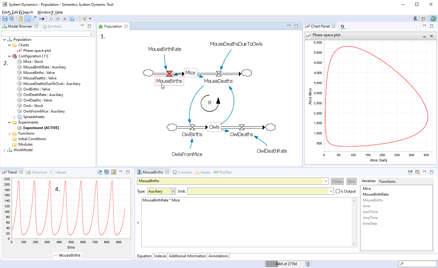
1 Diagram
Diagram is the area where you will graphically modify your model. Diagrams are built from elements that can be dragged from Symbols view or populated using shortcut keys.
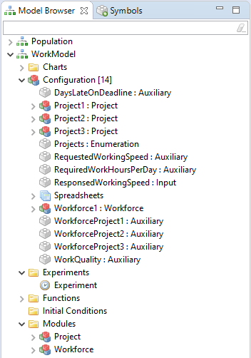
2 Model Browser
Model browser shows the structure of your model and all items related to it.
Symbols
Symbols view (stacked with the model browser) is used for dragging elements to diagrams.
3 Properties (MouseBirths in the image above)
Property view shows the selected variable's properties. Property view has a different layout depending on the type of the selected component. The view can also have different tabs depending on the component type. Basic tabs for variables are Equation, indices, and Additional information.
Console
Console view (stacked with the property view) shows console messages from the simulator. Console can be used for debugging models simulated using OpenModelica.
Issues
Issue view (stacked with the property view) shows the errors and warnings in all models.
Profiles
Profiles view (stacked with the property view) allows enabling/disabling some visual diagram effects.
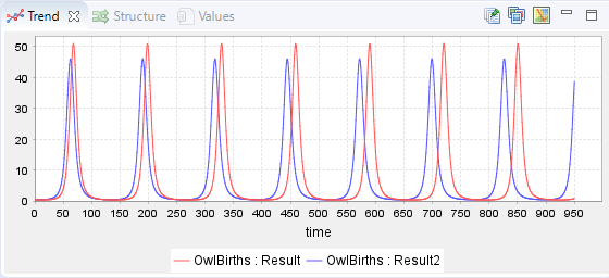
4 Trend
Trend view shows the graphical representation of the values of the selected value over time. For the trend to be shown, a simulation has to be run. The view shows always the results of the latest run, but you can save results of a simulation and show them in the same trend with results from another simulation.
Structure
The structure view (stacked with the trend view) can be used for analyzing the variable dependencies, loops, and the structure of the model.
Values
The values view (stacked with the trend view) shows the values of the selected value over time. For the values to be shown, a simulation has to be run.
5 Save and save as...
Save buttons can be used to export the selected model as .sysdyn file. The buttons save that model which is selected in the model browser or, if the focus is on the diagram, the model that is currently open on the diagram.
6 Diagram tool mode
With the diagram tool mode, you can select how the elements on the diagram are edited. The Lock mode prohibits editing diagram elements, the pointer mode allows moving and editing diagram elements, and with the dependency and flow modes arrows can be drawn using only mouse1 and mouse2.
7 Experiment controls
Experiment controls are shown when an experiment is active. Experiment is activated by double clicking an experiment in the model browser. With the experiment control, you can start simulation runs and save simulation results.
8 Perspectives

9 Chart Panel
Chart panel is able to house multiple charts at the same time. Charts are added to the panel by dragging from model browser.
TIP! If you accidentally close a view, you can reopen them from Window→Show View→Other...
TIP! Try dragging the views to different positions (e.g. the property view to the right pane).
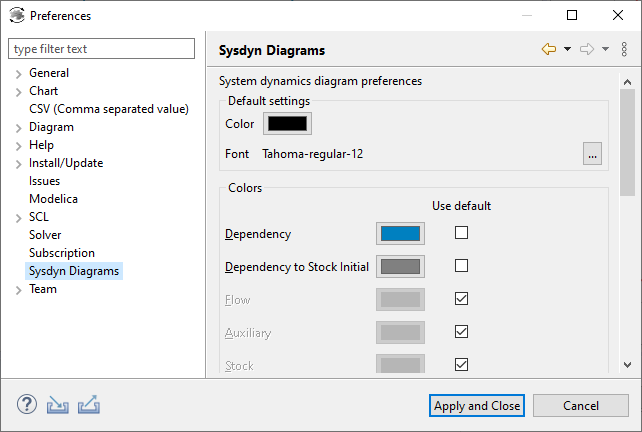
Global Preferences
Global preferences of Simantics System Dynamics are located under Window → Preferences. Feel free to browse the contents yourself. A few notable items on the list are described below.
| Category | Description |
|---|---|
| General → Keys | All keyboard shortcuts available. |
| Modelica | The location of OpenModelica solver on file system. |
| Solver | Solver to be used for simulation. OpenModelica or internal custom solver (experimental) can be selected. |
| Sysdyn Diagrams | Sysdyn Diagrams allows customize default colors and fonts of diagram elements. |
Modelling
Basic Modelling
Basic modelling functions enable you to create and configure models. System dynamics modeling is basically pretty simple, so with these instructions you can build small and also very large models. The tricky part is writing all the expressions and adjusting the model so that it actually tells you something.
Creating a new model
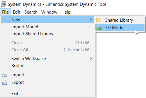
Start a new model by right-clicking the model browser and selecting New → Model or from the main menu File → New → SD Model.
Creating a new module type
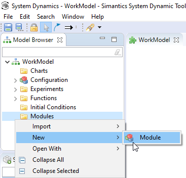
Create a new module type by right-clicking on the Modules-folder and selecting New → Module type. This creates a new module type that you can populate to your other modules and the model configuration.
Configuring a model
Model configuration can be opened by double clicking Configuration in the model browser.
Configuring modules
Configuration of a module type can be opened by double clicking the module type you want to configure. You can also open the configuration of a module from a diagram, when a module has been populated to that diagram, by right-clicking the module and selecting Show Module. When opening modules from diagram, the opened diagram knows to which diagram the module has been populated and can show the connections between the modules. Keep in mind that when making changes to a module, the changes apply to all instances of the respective module type!
Populate variables
You can drag variables to a diagram from symbol view. You can also populate variables using shortcut keys. Variables can be divided into multiple lines by resizing the variable on diagram.
Populate modules
Modules are populated from the model browser. Just drag the module you want to populate from the Modules folder to a diagram.
Create connections
There are two types of connections: dependencies and flows. Both are created basically the same way. Hold Alt down and click on a variable. Left click starts a dependency, right click starts a flow. Both are ended to another variable with a left click. Dependencies and flows can also be created without Alt key by selecting dependency or flow mode on the toolbar.
Flows can also be started and ended to an empty spot in the diagram. If there is no start or end variable, a cloud will be created. Also if start or end is not a valve, a new valve is created in the middle of the flow.
There are some restrictions on what connections can be made, but don't worry, the user interface won't let you do connections that are not allowed.
Connections between modules
Outside the module
You can connect variables to modules like this:
MODULE -----> INPUT
or
ANY VARIABLE -----> MODULE
This is just the visual configuration, but you need those connections to really connect variables in the module's properties.
In the Inputs tab stacked under Module Properties you can select which variables you connect to inputs inside the module. In the Outputs tab you can select which variables you lift from the module to inputs outside it.
Inside the module
Input variables get values from outside the module.
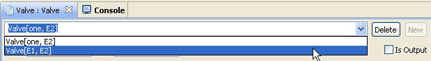
Output variables send their values outside the module. To make a variable output its values, from the properties view make sure the Is Output checkbox is ticked.
Configure variables
Select a single variable from diagram or model browser. The properties of the variables are shown in the properties view where you can also modify them.
Export model
To export your model to a file, select your model from the model browser, right-click and from the context menu choose Export→Model. Select the folder where to export your model, give the file a name and press Save. You do not need to export a model to Save it, the model is automatically saved in your database. Export can be used, for example, to create different versions of a model, create backups or to transport a model to another database.
Import model
Select File→Import Model, browse to your .sysdyn file and select open. The model is added to your model browser.
Export module
To export a module to a file, select the module from the model browser, right-click and from the context menu choose Export→Module. Select the folder where to export your model, give the file a name and press Save. Module export can be used, for example, to transport a module to another model or another database.
Import module
Right-click the Modules folder of a model and select Import→Module. Browse to your .sysdynModule file and select open. The module is added to your model.
Model Properties
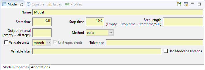
Model properties can be viewed by selecting either the model or its configuration on the model browser.
| Property | Description |
|---|---|
| Name | The name of the model |
| Start time | The start time of the simulation. |
| Stop time | The stop time of the simulation. |
| Step length | The length of the simulation step. |
| Output interval | Interval of witch the simulation result is presented. If the field is left empty, all steps of the output are presented. |
| Method | The simulation solver (only OpenModelica). |
| Validate units | Unit validation on/off. If unit validation is enabled, the unit of the simulation time is selected from the pull-down menu. |
| Unit equivalents | Define if different forms of predefined units are considered equal (e.g. dollars = dollar = $) in unit validation. |
| Tolerance | Integrator error tolerance (only OpenModelica) |
| Variable filter | Define which variables are presented (only OpenModelica) |
Special Variables
Auxiliary and valve variables have two special types: WithLookup and Delay. These types are selected from Type drop down menu in the variable's properties. The variable types offer more specific functionalities than normal variables, but the same functionality could be achieved using normal variables.
WithLookup
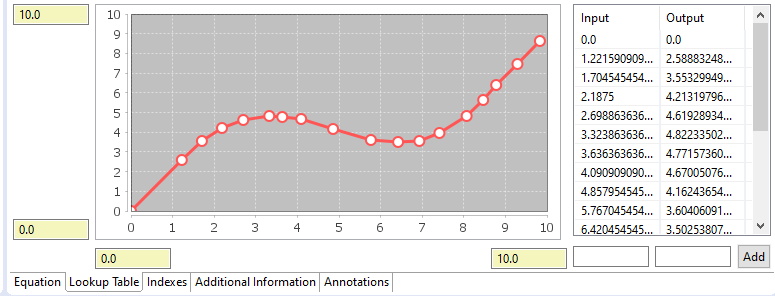
WithLookup variable has two equation fields, WithLookup and Lookup table. Lookup table has a table from which the value of the variable is interpolated using the value of WithLookup field.
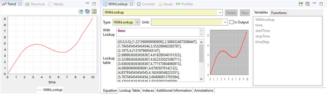
You do not need to manually input the Lookup table. WithLookup variable type offers an additional Lookup table tab in the property view. In this view you can add and modify points in the lookup table. Points can be added either by clicking on the chart or by using the input fields and Add button. Points can be modified by dragging them on the chart or modifying values in the table. Points are removed by clicking them with right mouse click.
Delay
Delay variables build equations for Nth order delays. Users can set the equation for the value that is to be delayed, the time and order of the delay and a possible start value. If start value is empty, the start value is set automatically.
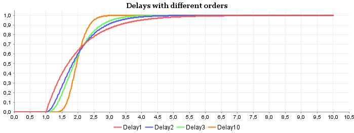
Different order delays have slightly different curves when a step change is triggered. The example picture below shows a step change from 0 to 1 at time 1 with four different delays: 1st, 2nd, 3rd and 10th order delays.
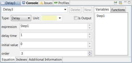
For further information on how the delays work, you can look at the equations that are created by the delay variable. Below is a third order delay. Delay3 is the actual variable that is seen by users. DelayClass has as many level (LV) variables as the order of the delay is.
Definitions:
Real Delay3;
Delay3_delayClass Delay3_delayClass_instance(initialValue = 0, delayTime = 1);
class Delay3_delayClass
  parameter Real DL = delayTime/3;
  parameter Real delayTime;
  parameter Real initialValue;
  Real delay0;
  Real LV1(fixed=true, start=initialValue * DL);
  Real delay1;
  Real LV2(fixed=true, start=initialValue * DL);
  Real delay2;
  Real LV3(fixed=true, start=initialValue * DL);
  Real delay3;
equation
  der(LV1) = - delay1 + delay0;
  delay1 = LV1 /DL;
  der(LV2) = - delay2 + delay1;
  delay2 = LV2 /DL;
  der(LV3) = - delay3 + delay2;
  delay3 = LV3 /DL;
end Delay3_delayClass;
The above definitions can be seen as a line of stocks and valves. The first valve, delay0, is given the value of the delayed expression. Delay3 is given the value of the valve that is coming from the last stock.
Equations:
Delay3_delayClass_instance.delay0 = Step1;
Delay3 = Delay3_delayClass_instance.delay3;
Shortcut and Control Keys
Shortcut keys for configuring a model on diagram.
| Key | Action |
|---|---|
| Esc | Cancel operations (e.g. connection and rename). |
| Shift + A | Hover Auxiliary at the cursor position, populate with left mouse button. |
| Shift + S | Hover Stock at the cursor position, populate with left mouse button. |
| Shift + C | Hover Cloud at the cursor position, populate with left mouse button. |
| Shift + V | Hover Valve at the cursor position, populate with left mouse button. |
| Shift + I | Hover Input at the cursor position, populate with left mouse button. |
| Shift + G | Hover Shadow (Ghost) variable at the cursor position, populate with left mouse button. |
| Alt + left mouse button | Start an arrow from a variable. End to another variable by clicking left mouse button. |
| Alt + right mouse button | Start flow from a variable. End by clicking left mouse button. If a flow is not started or ended on to a variable, a cloud will be created to that end. If a new flow does not have a valve at either end, a valve will be created in the middle of the flow. |
| Delete | Remove selected variables |
| F2 | Rename selected variable |
| Ctrl + left mouse button | Select multiple variables |
| Mouse wheel or + or - | Diagram zoom |
| drag(mouse3) | Diagram pan |
| drag(shift + right mouse button) | Diagram pan |
| ↓, ←, ↑, → (arrow keys) | Diagram pan |
| Ctrl + C | Copy selected elements |
| Ctrl + X | Cut selected elements |
| Ctrl + V | Paste copied or cut elements |
| Ctrl + F | Find element in current diagram or all models |
| G | Show / hide grid |
| R | Show / hide ruler |
| 1 | Fit diagram contents to screen |
| Ctrl + Space | Content assist in equation editor |
Other shortcut keys can be found selecting Window → Preferences from the main menu. Keys are located in General → Keys.
Unit Validation
Unit validation is useful for finding errors in the model. Unit validation checks the consistency of units. To use this feature you need to define units for every variable used in the model. If a variable is dimensionless, use 1 as the unit. In certain constructs, a dimensionless variable can be used as "a wild card", e.g., adding a dimensionless variable with a dimensioned one is OK.
Common error sources of unit validation include the following. The respective issues are shown in the picture below.
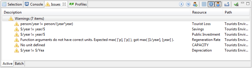
The equation of a variable yields a different unit than that defined for the variable.
Two variables which have different units are added (+), subtracted (-), or compared (>, <, =, ...).
The output unit of a function is used in an inconsistent manner. (The unit validation for the output unit of a function behaves equivalently to the unit of a variable.)
A function is called with an argument of a prohibited unit.
A variable has an empty unit.
A variable has a misspelled unit.
Unit validation is enabled for a model by selecting the model or its configuration on the model browser and enabling "Validate units" on the properties tab. The unit warnings are shown on Issues view and, supposing the respective profile has been enabled, on the diagram as well. Warnings from unit validation do not prevent simulation.
For models that have stocks (i.e., integration), the simulation time unit must be selected from the pull-down menu next to the "Validate units" checkbox in Model Properties tab.
Unit validation can also cope with certain different forms of units, e.g., you can write dollars, dollar, or $ and the validator considers these equal. This functionality can be disabled from Model Properties tab checkbox "Unit equivalents".
As there may be cases for which the unit validation is for some reason not working as desired, the unitCast() function can be used in the equation of a variable to cast the unit of any expression within the equation to a wildcard. E.g., if expression
Aux1 + time
yields a warning, it can be fixed be changing the expression to
unitCast(Aux1) + time
in which case the unit of the expression is that of time, or to
Aux1 + unitCast(time)
in which case the unit of the expression is that of Aux1.
Diagram Profiles
Diagram profiles allow selecting which visual effects are enabled. Currently the following profiles can be used:
Default
Issue warnings
When enabled, an error or a warning symbol is attached to diagram elements in which there are errors or warnings (usually in the equations).
Shadow variable visualizations
When enabled, the original and all the shadow variables are highlighted when one is selected.
Simulation Playback
Playback Colors
When enabled, colors of the elements on diagram change during a playback experiment.
Debugging a model
If you find yourself with a model that doesn't simulate or has bizarre behavior, there are several places to look for clues for what went wrong. Firstly, if you got an error message and can't infer the problem straight from the message, look at the issues view if it can tell you what is wrong in different words. If you know how to read Modelica code, right click Configuration under the broken model and choose Open With → Modelica Code Viewer. The tool works by generating Modelica code from the graphical model and then solving it. Therefore, if something is broken it means that there is a problem with the generated Modelica code (or, very rarely, a bug in the solver you are using). You can also refer to the list below, if you still find yourself stuck.
Some of the most common errors include:
In a model that uses modules, you forget to connect inputs and/or outputs in the module properties
You forgot to add an enumeration to a variable, i.e. trying to put a vector to a scalar variable (or vice versa)
You increased the enumeration indices you are using, but forget to update a variable that depend on it
You wrote a custom Modelica function, but it is broken
You are comparing two numbers for equality while using OpenModelica solver (forbidden, allowed by the internal solver)
You have a variable that refers to itself in the equation, making the solver unable find an initial value
If you are using OpenModelica solver it can be very useful to google error messages printed in the console of the tool.
Visual model elements
The visual appearance of the elements on diagram can be modified in various ways. In addition, the tool has comment symbols which do not affect simulation but help the understandability of models.
Fonts and colors
Fonts and colors of diagram elements can be changed by right-clicking the element and selecting Font... The default fonts and colors for each diagram element type can be changed in Window → Preferences → Sysdyn Diagrams.
Dependency properties
Dependency arrow properties can be changed on the property view:
Polarity
Polarity sign can be used to indicate whether the dependency increases or decreases the variable it is pointing to. The polarities serve no function for simulation, however, they are used in loop type automatic determination.
Location
Location of the polarity mark
Arrowhead
Toggle for showing arrowhead
Delay mark
Delay mark is a visual cue for helping understandability of the dynamics of the model when there are (information) delays. A delay mark is usually added to the dependency arrow when the effect the tail of the dependency has on the head of the dependency is delayed.
Line thickness
Thickness of the arrow
Loops
A loop element is a graphical component for highlighting feedback loops in a model. Usually the most interesting feedback loops that affect the behaviour of the model most are marked with a loop symbol.
Loop Items
The loop of variables which the loop symbol refers can be selected for visualization purposes.
Comment
Comment inside the loop. Usually characters 'B' and 'R' are used to denote balancing and reinforcing loops, respectfully. A feedback loop is reinforcing if and only if it has an even number of negative dependencies. Selecting 'Auto' determines automatically the type of the loop.
Direction of Rotation
Direction to which the loop rotates on diagram.
Comments
Comments are just strings of text.
Simulation
Experiments
There are three different ways for simulating a model. Different simulations are represented as different types of experiments in Simantics System Dynamics. Currently some of the experiment and solver combinations are still in development.
Experiments are created from the context menu of experiments folder in a model.
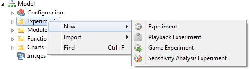
Double-click on an experiment activates it and displays experiment type specific controls in the main tool bar.
Normal simulation
Experiment is the basic simulation type. It simulates a model from start time to end time and results can be viewed after the simulation has been run. Works on both the internal and OpenModelica solvers.
Game simulation
Game simulations allow simulating an arbitrary number of steps, changing parameter values and continuing simulation with the new values from where it previously ended. Works on the internal solver, OpenModelica version still in development.
Simulation playback
Simulation playback works essentially as the basic experiment, but it offers some additional visualization options. Works on both solvers.
Sensitivity analysis simulation
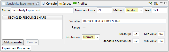
Sensitivity analysis allows running multivariate Monte Carlo simulations with different parameter value sets and to visualize how much the simulation result depends on changes in the selected parameters. Works on OpenModelica solver, internal solver implementation still in development.
| General | - |
|---|---|
| Name | The name of the sensitivity analysis experiment. Displayed in e.g. model browser. |
| Number of runs | The total amount of individual simulation runs |
| Method | The method of how the parameter values are selected from the distribution(s). Selecting "Random" yields pseudo-random values, i.e., randomly selected from the distribution(s). Selecting "Halton" yields a quasi-random Halton sequence of values selected deterministically to represent the distribution(s) better than a pseudo-random series. |
| Seed | The seed number for pseudo-random generator |
| Add parameter | Adds a new parameter to be varied |
| Remove | Removes a parameter |
| Parameter properties | - |
| Variable | The full path of the variable of which value is varied. This field has content assistant, which shows the possible variables as you type. |
| Range | Used with multidimensional values to select which dimensions are varied. |
| Distribution | Probability distribution for the varied parameter. "Normal" is for truncated normal distribution and "Uniform" for uniform distribution. With "Interval" the values have equal intervals between each other and are selected in increasing order. In multivariate sensitivity analyses, it is recommended to select either "Normal" or "Uniform". |
| Distribution properties | - |
| Min value | Minimum value of the distribution |
| Max value | Maximum value of the distribution |
| Mean | Mean of the normal distribution |
| Standard deviation | Standard deviation of the normal distribution |
Solvers
Simantics System Dynamics allows using the multiple solvers provided by OpenModelica, like Euler, Runge-Kutta, DASSL, etc. OpenModelica is currently the main simulation environment behind the tool and all functionalities are supported with OpenModelica.
Alternatively to OpenModelica, an internal custom Modelica solver is included in Simantics System Dynamics. The custom solver is currently at an experimental state, and thus all functionalities of the tool are not yet supported, e.g., only the basic experiment can be run with it. The advantage of the custom solver is, however, that simulation is usually a lot faster than with OpenModelica. Try out yourself which solver suits best for your needs.
The solver can be changed in Windows → Preferences → Solver.
Simulation Result and Model Structure Analysis
Simulation results can be viewed as trends in the trend view or as plain numbers in the values view. The views display results of variables that are selected in the workbench. Users can also create custom charts.
Model structure can be examined in the Structure view. There are three options: dependency structures of individual variables, the complete hierarchy structure of the model, or the feedback loops which individual variables belong to.
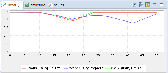
Trend
Shows you the values of the selected variable(s) graphically over the simulation time. You can modify the trend and zoom it using the context menu (right-click) of the trend. You can also export the trend using controls in the upper right corner.
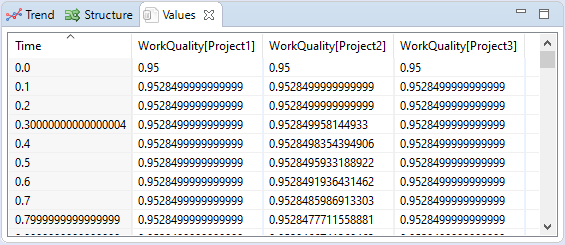
Values
Shows you the values of the selected variable(s) in a table form. If the value has a star (*) at the end, it means that the value is an approximate. There is no value for that variable for the given time step. Selected values can be copied to other software in csv format.
Compare results
You can compare different results of the same model by saving simulation results and displaying the saved results side by side with other results. This functionality currently only works for the OpenModelica solver, internal solver implementation is in development. You can save your results after simulating by clicking the Save Results button:

on your experiment controls. The saved results appear to model browser under the active experiment. To show the results on trends and tables, double click on the result to activate it.
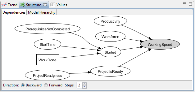
Dependencies
Dependencies display which variables affect and which are affected by the selected variable. The direction and number of steps that are traveled from the selected variable can be configured at the bottom of the view.
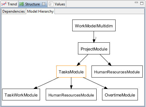
Model Hierarchy
Model Hierarchy displays the hierarchical structure of the model. The module type where a selected variable is located is highlighted.
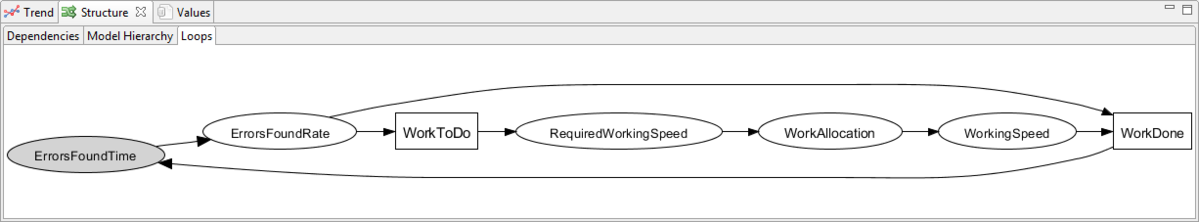
Loops
Loops display all feedback loops which the selected variable belongs to.
Custom Charts
Custom charts are user-defined displays of simulation result data. They can be used and re-used in various places. The four types of custom charts (line, sensitivity, bar, and pie charts) provide model developers means for examining and developing their models and communicating the simulation results to others.
Custom charts are created to the Charts folder in model browser.
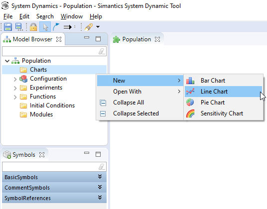
Charts are configured the same way as variables: first select the chart from model browser and then configure it in the property view. Charts can be viewed in the same active trend view as any variable by selecting the chart from model browser. In addition to trend view, charts can be populated directly to the model diagram by dragging them from the model browser. Charts can also be added to a separate chart panel which can contain multiple charts.
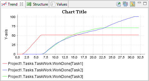
Line Chart
Line chart shows the time series of a variable. It is capable of displaying multiple multi-dimensional variables at the same time. Simulation playback mode adds a marker to the chart to display the current time in playback simulation. Below is an example chart and its settings.
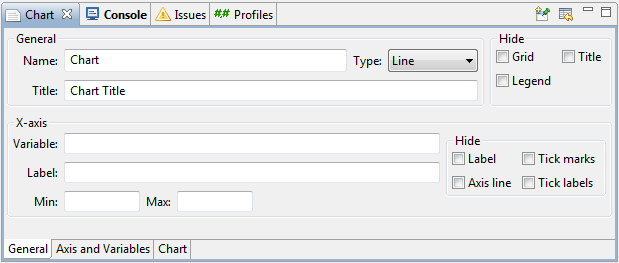
| General | - |
|---|---|
| Name | The name of the chart. Displayed in e.g. model browser |
| Title | The title of the chart. Displayed in the chart |
| Type | Line chart (default) or area chart |
| Hide | Options to hide chart grid, title or legend |
| X-axis | - |
| Variable | A variable that is used as the x-axis variable. The default variable is time and it needs not to be typed in the field. |
| Label | Optional other label for the variable than its name |
| Min | Minimum value of the x-axis |
| Max | Maximum value of the x-axis |
| Hide | Options to hide x-axis label, line, tick marks and tick labels |
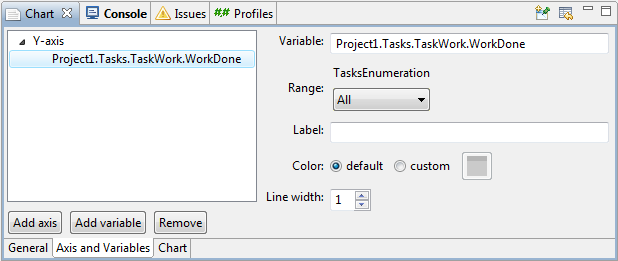
| Variable | - |
|---|---|
| Variable | The full path of the variable. This field has content assistant, which shows the possible variables as you type. |
| Range | If the variable has multiple dimensions, this field allows to select, which dimensions are displayed. It is also possible to sum the variables in the dimensions. |
| Label | Optional label for the variable. If label is empty, the variable name is displayed. |
| Color | Color for the lines of this variable |
| Line width | The width of the lines drawn for this variable |
There are also configuration options for y-axis. They are displayed when an axis is selected in the Axis and variables tab.
| Y-axis | - |
|---|---|
| Label | Label of the axis |
| Min | Minimum value in the axis |
| Max | Maximum value in the axis |
| Color | The color of the axis lines, ticks and labels |
| Hide | Options to hide parts of the axis: label, axis line, tick marks, tick labels |
Sensitivity Chart
Sensitivity chart shows the time series of a variable with confidence bounds. Below is an example chart and its settings. The general settings are defined similarly to those of a line chart explained above.
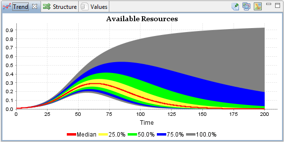
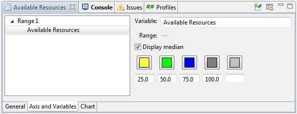
| Axis and Variables | - |
|---|---|
| Variable | The full path of the variable. This field has content assistant, which shows the possible variables as you type. |
| Range | If the variable has multiple dimensions, this field allows to select, which dimensions are displayed. It is also possible to sum the variables in the dimensions. |
| Display median | Display the median value of the variable at each time step. |
| Confidence bounds and colors | The confidence bounds in percentages and colors for them. |
There are also configuration options for y-axis. They are displayed when an axis is selected in the Axis and variables tab.
| Y-axis | - |
|---|---|
| Label | Label of the axis |
| Min | Minimum value in the axis |
| Max | Maximum value in the axis |
| Color | The color of the axis lines, ticks and labels |
| Hide | Options to hide parts of the axis: label, axis line, tick marks, tick labels |
Bar Chart
Bar charts display variables in a certain point in time. The point can be defined for the complete chart in chart's general settings and individually for each variable in variable's settings. If no time is defined, the last simulation step is shown in game or normal simulation mode. Playback mode displays the current playback time.
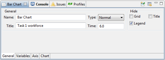
| General | - |
|---|---|
| Name | The name of the chart. Name is displayed in model browser. |
| Title | The title of the chart. Title is displayed in the chart, if not hidden |
| Type | Normal or stacked. Normal type displays all variables in separate bars. Stacked mode is able to display one-dimensional array variables in stacks. |
| Time | A general time setting for the entire chart. The values at this time are displayed in the chart |
| Hide | Option for hiding grid, title and Legend. Legend is hidden by default since it only contains the information that the current simulation is displayed. |
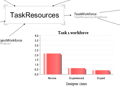
Charts can be added to model diagrams simply by dragging the chart from model browser to diagram.
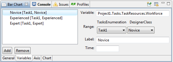
| Variable | - |
|---|---|
| Add / Remove | Add or remove variables |
| Variable | The full path of the variable. This field has content assistant, which shows the possible variables as you type. |
| Range | If the variable has multiple dimensions, this field allows to select, which dimensions are displayed. It is also possible to sum the variables in the dimensions. |
| Label | Optional label for the variable. If label is empty, the variable name is displayed |
| Time | The time for which the value of this variable is displayed. If this is empty, a general (or default) value of the time is used. |
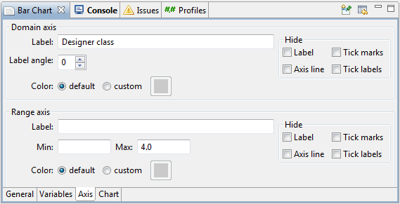
| Domain axis | - |
|---|---|
| Label | An optional label for x axis |
| Label angle | Axis labels can be displayed in an angle. This value determines the angle in degrees. |
| Color | The color of the axis line, tick lines and labels |
| Hide | Options for hiding axis label, line, tick marks and tick labels |
| Range axis | - |
| Label | An optional label for y axis |
| Min | Minimum value of y axis |
| Max | Maximum value of y axis |
| Color | The color of the axis line, tick lines and labels |
| Hide | Options for hiding axis label, line, tick marks and tick labels |
Pie Chart
Pie charts display proportions of variables at a certain time. The time, similar to bar charts, can be configured for the whole chart and individually for each variable. If no time is configured, the value at the latest time step (or the time of simulation playback) is displayed.
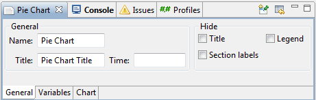
| General | - |
|---|---|
| Name | The name of the chart. Displayed in e.g. model browser |
| Title | Title The title of the chart. Displayed in the chart |
| Time | A general time setting for the entire chart. The values at this time are displayed in the chart |
| Hide | Options for hiding title, section labels and legend |
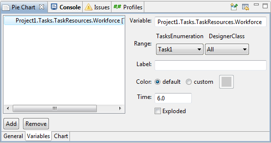
| Variables | - |
|---|---|
| Add / Remove | Add or remove variables |
| Variable | The full path of the variable. This field has content assistant, which shows the possible variables as you type. |
| Range | If the variable has multiple dimensions, this field allows to select, which dimensions are displayed. It is also possible to sum the variables in the dimensions. |
| Label | Optional label for the variable. If label is empty, the variable name is displayed |
| Color | Color for the sector of this variable |
| Time | The time for which the value of this variable is displayed. If this is empty, a general (or default) value of the time is used. |
| Exploded | If set, the sector(s) of the variable(s) are "exploded" away from the center of the pie chart |
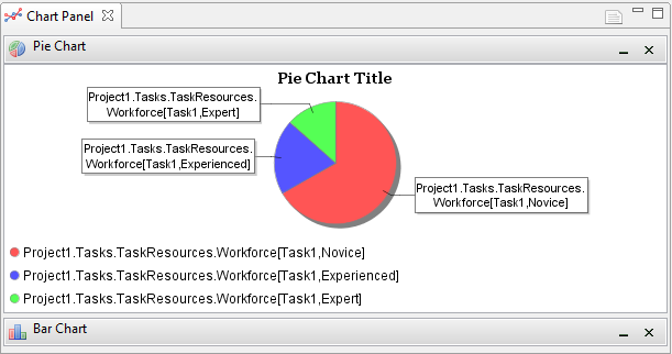
Chart Panel
Chart panel is able to house multiple charts at the same time. Chart panel is a normal view in the workbench, which means it can be resized and located anywhere in the workbench. Eclipse also allows detaching the tab completely from the workbench, which means that the chart panel can be dragged to another screen.
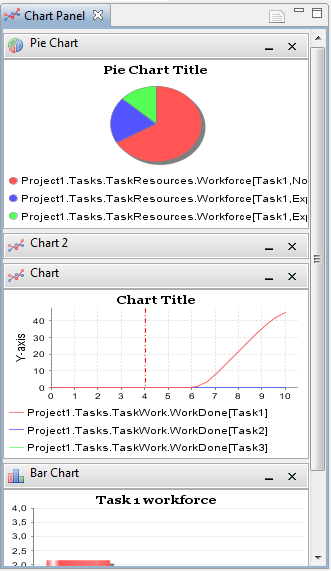
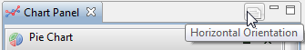
Chart panel can be either horizontally or vertically oriented. Different orientations help in configuring the workbench perspective.
Charts are added to the panel by dragging from model browser. The order of the charts is easily changed by dragging charts from their header. Charts can be minimized or completely removed from the buttons in their headers.
By default, chart panel is hidden in the upper-right corner of the system dynamics perspective.
Multidimensional Variables
Modeling
Models with multidimensional variables look just like any other models. The structure of the models is replicated giving multiple indices to variables. For users with programming background, notation Variable may be familiar. In system dynamic modeling we need to give names to the indices. Instead of using numbers to define the indices, like in normal programming, we use enumerations. The steps to create a model with multidimensional variables are as follows (with examples):
1 Create the model structure
Model with multidimensional variables looks just like any other model.
2 Create Enumerations and define the indices
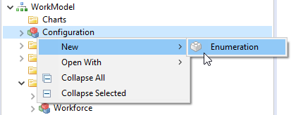
Enumerations are created by right-clicking configuration and selecting New→Enumeration.
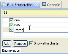
Define enumeration indices by adding as many indices as you want. Rename the indices by selecting them and then clicking on them again.
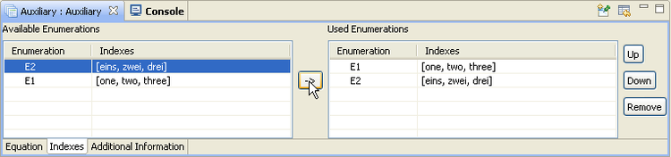
3 Add Enumerations for variables
Select the variable that you want to be multidimensional. From the indices -tab in the property view, move the wanted enumerations to the right. The order of the enumerations does matter.
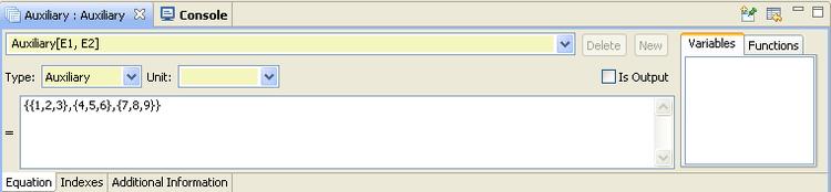
4 Define equations for all possible indices
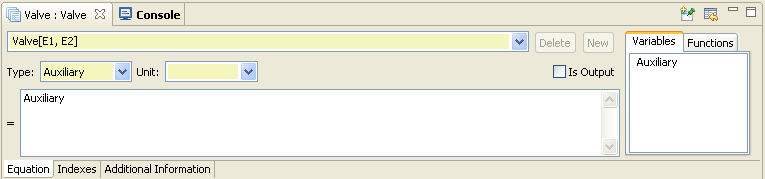
Multidimensional variable can be thought as a multidimensional table. Each cell of the table needs to have an expression or a value. A cell cannot have multiple definitions. All cells can be defined in one expression like in the following example. E1 and E2 have both three indices, so the resulting definition can be {{1,2,3},{4,5,6},{7,8,9}}.
Expressions
Values for all cells in the variable matrix can be defined in a single expression.
In many situations, it is however more clear to define separate expressions for each cell or blocks.
1 Define range for the expression
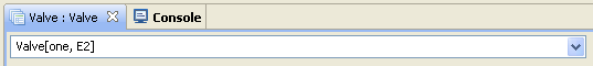
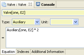
2 Define the expression (dimensions of the defined range and the result of the expression must match!)
3 Create a new expression
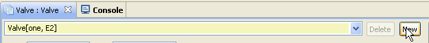
4 Select the new expression
Repeat until there is value for each cell. There must be exactly one value for each cell.
Array Slices
Many times it is useful to access a slice of a multidimensional variable. In this chapter, we will use the following example variable:
 enumeration E1 = one, two, three
 enumeration E2 = eins, zwei, drei
 Auxiliary[E1, E2] = {{1,2,3},{4,5,6},{7,8,9}}
The whole variable can be accessed in three different ways:
AuxiliaryAuxiliary[E1, E2]Auxiliary[:, :]
The following explains different methods for accessing parts of the variable
 // Single cell
 Auxiliary[one, eins] = 1
 // Slices
 Auxiliary[one, E2] = {1,2,3}
 Auxiliary[E1, zwei] = {{2},{5},{8}}

 // In addition to single cells and the whole enumeration range, a subrange of the enumeration can be used
 Auxiliary[two : three, E2] = {{4,5,6},{7,8,9}}
 Auxiliary[one : two, zwei : drei]  = {{2,3},{5,6}}
The syntax for accessing parts of variables can be used in both expression range definitions and in expressions.
Arithmetic Operators
Arithmetic operations are defined in Modelica. Below are examples of different operations.
Addition and substraction
Addition and substraction are calculated elementwise
 {1,2,3} - {0,2,3} = {1,0,0}
 {{2,2},{4,4}} + {{8,8},{1,1}} = {{10,10},{5,5}}
 {1,2,3} - {1,2} = ERROR! Different array sizes
Division
Division with a scalar
 {5,10,15} / 5 = {1,2,3}
 5 / {5,10,15} = ERROR! not allowed
Division with an array
 {1,2,3} / {1,2,3} = ERROR! not allowed

 // Elementwise
 {1,2,3} ./ {1,2,3} = {1,1,1}
Multiplication
Multiplication with a scalar
 {1,2,3} * 2 = {2,4,6}
 5 * {1,2,3} = {5,10,15}
Matrix multiplication with an array
 {{3,4},{5,6}} * {1,2} = {11,17}
 {{3,4},{5,6}}  * {1,2,3} = ERROR! incompatible array sizes

 //Elementwise
 {1,2} .* {1,2} = {1,4}

 Real[3,2] c = {{1,2},{3,4},{5,6}};
 Real[2,2] d = {{3,4},{5,6}};
 Real[2,2] cd;
 cd = c[2:3, :] .* d; // Result: {{9,16},{25,36}}
Power
Elementwise power of array variable
{1,2} .^ 2 = {1,4}
Built-in Modelica Functions
Modelica has some built-in functions that help using multidimensional variables. You can find the functions under any model inside the folder Functions→Built-in Functions. This chapter introduces some of the built-in functions.
Dimension and size functions
We will use the same example variable as previously.
 enumeration E1 = one, two, three
 enumeration E2 = eins, zwei, drei

 Auxiliary[E1, E2] = {{1,2,3},{4,5,6},{7,8,9}}
ndims(A)
The number of dimensions in array A
ndims(Auxiliary) = 2
size(A, i)
The size of dimension i in array A
size(Auxiliary, 2) = 3
size(A)
A vector of length ndims(A) containing the dimension sizes of A
size(Auxiliary) = {3,3}
Construction functions
In addition to normal array constructing, a special construction functions can be used.
zeros(n1,n2,n3,...)
An array full of zeros with dimensions n1 x n2 x n2 x ...
zeros(2, 2) = {{0,0}, {0,0}}
ones(n1,n2,n3,...)
An array full of ones with dimensions n1 x n2 x n2 x ...
ones(2, 2) = {{1,1}, {1,1}}
fill(s,n1,n2,n3)
Like zeros() and ones(), but with user defined value (s) for array elements.
fill(3,2,2) = {{3,3}, {3,3}}
identity(n)
Creates an n x n integer identity matrix with ones on the diagonal and all other elements zero.
 identity(3) =
   1 0 0
   0 1 0
   0 0 1
diagonal(v)
Constructs a square matrix with elements of vector v on the diagonal and all other elements zero.
 diagonal({1,2,3}) =
   1 0 0
   0 2 0
   0 0 3
linspace(x1,x2,n)
Constructs a Real vector from x1 to x2 with n equally spaced elements.
linspace(2,5,4) = {2,3,4,5}
Reduction functions
Reduction functions reduce arrays to scalars.
min(A)
Returns the minimum value in array A.
 Real A = {{1,2},{3,4}}
 min(A) = 1
max(A)
Returns the maximum value in array A.
 Real A = {{1,2},{3,4}}
 max(A) = 4
sum(A)
Returns the sum of values in array A.
 Real A = {{1,2},{3,4}}
 sum(A) = 10    // 1 + 2 + 3 + 4
product(A)
Returns the product of values in array A.
 Real A = {{1,2},{3,4}}
 product(A) = 24   // 1 * 2 * 3 * 4
Using functions with iterators
Functions min(A), max(A), sum(A) and product(A) reduce arrays to scalars. When you use multidimensional variables, you will most probably like to reduce less dimensions. This can be achieved using iterators with reduction functions. The result is constructed as an array, if curly brackets {} are used to enclose the expression.
 enumeration E1 = one, two, three
 enumeration E2 = eins, zwei, drei
 Auxiliary[E1, E2] = {{1,2,3},{4,5,6},{7,8,9}}

 AuxiliarySum[E1] = {sum( Auxiliary[ i , E2 ] ) for i in E1} // Result: {6, 15, 24}

 /* Same as:
 {sum(Auxiliary[one, E2]), sum(Auxiliary[two, E2]), sum(Auxiliary[three, E2])}
 {sum({1,2,3}), sum({4,5,6}), sum({7,8,9})}
 */
One expression can have multiple iterators. The Modelica specification defines the following format, but it is NOT yet supported in OpenModelica:
{sum(Array[ i, j, E3]) for i in E1, j in E2} // Dimensions reduced from 3 to 2
To use multiple iterators, use the following format (NOTE the reversed order of iterators!):
{{sum(Array[ i, j, E3]) for j in E2} for i in E1} // Dimensions reduced from 3 to 2
The range doesn't have to be the whole enumeration. Subranges can also be used.
 {sum( Auxiliary[ i , eins : zwei ] ) for i in E1.one : E1.two} // Result: {3, 9}

 /* Same as
 {sum(Auxiliary[one, eins : zwei]), sum(Auxiliary[two, eins : zwei])}
 {sum({1,2}), sum({4,5})}
 */
Simulation Results
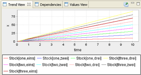
Multidimensional variables provide multiple results for the same variable. One result for each index. The trend view clutters very quickly when you add dimensions to the variables.
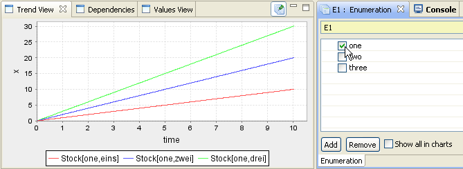
The clutter can be reduced by selecting which enumeration indices are shown in charts. Select an enumeration and tick the indices that you want to show. The same settings apply to each variable that uses the enumeration. This way you can follow an interesting index throughout the model.
Array Variables in Modules
Replaceable enumeration inside a module
You can also use array variables inside modules. Enumeration need to be defined separately for each module type and added to all necessary variables, also inputs and outputs (see Modeling).
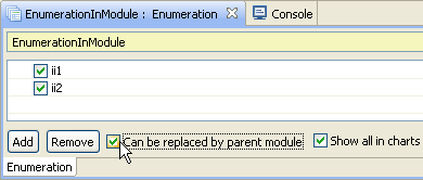
When defining a module, modeler may not want to restrict the size of the array variable. In many cases the same module structure could be used for both large and small arrays. For example if the module is a project, a project may have three or even twenty phases. In this case the enumerations inside modules need to be set as replaceable.
In this example, the original enumeration that the modeler used had two indices. We are using an instance of this module, but we need to use array variables that have three indices instead of two. We are using two variables and an instance of the module.
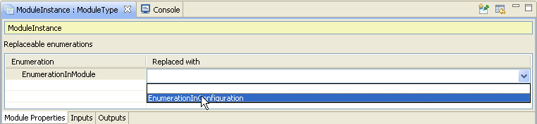
Module configuration for replacing enumerations inside the module
In the parent configuration, we have used an enumeration with three indices in the two variables.
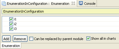
Enumeration in the parent configuration that will replace the enumeration in the module
The replacement can be defined in the properties of the module instance. When the module instance is selected, a table with all the replaceable enumerations is shown. By clicking on the cell next to the enumeration, a drop-down box is shown with all the enumerations in the parent module. If an enumeration is selected, it will replace the enumeration inside the module during simulation. The replacement will not, however, show elsewhere in the model.
Enumeration in the parent configuration that will replace the enumeration in the module
When creating replaceable enumerations in modules, modelers need to be very careful. Direct references to single enumeration elements are not allowed, since the enumeration elements will change, if the enumeration is replaced for simulation!
Functions
Modelica provides a convenient way to use functions in your models. You can create your own functions, export and import complete function libraries and share function libraries to be used in all of your models.
Creating Functions
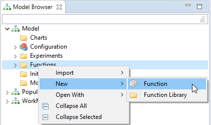
You can create new functions to the Functions -folder in your model or to function library folders. Right-click on the folder and select New→Function.
Functions that can be found from Functions -folder can be used in your variable definitions.
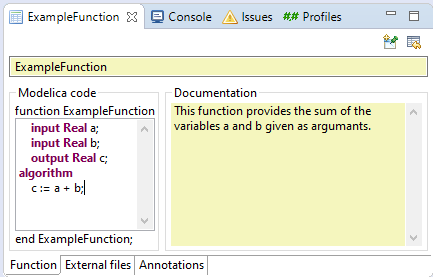
Functions are defined using Modelica language. The variables used in the function are defined in the declaration section. Function needs an output and an arbitrary number of inputs. Modelica specification enables use of multiple outputs, but this feature is not supported. The inputs are given in the same order as they are used in calling the function.
Algorithm section defines the actual functionality of the function. In algorithm sections you must use assignments ":=" instead of just plain "=". All the assignments are calculated in the order they are written.
Also, take note that creating new lines in the Modelica code text box is done via shift+enter.
Below is an example of a simple function. For more examples, see the built-in functions provided with the tool and Modelica specifications.
Function Libraries
Functions can be collected into libraries. This is a good way of organizing your functions. If function is located in a library, you need to append the library name to the function call (e.g. ExampleFunctionLibrary.ExampleFunction(arg1, arg2)). With libraries, you can also have functions with same names (e.g. library1.func(arg) and library2.func(arg)).
There are three types of function libraries: normal function library, built-in function library and shared function library. Normal function libraries can be created to a model and are available only in that model. Built-in libraries are available in all models and calls to built-in functions should not include the library name. Shared functions are available to all models in your workspace, but you need to enable them to each model individually.
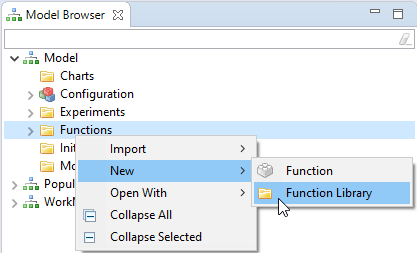
Create a new function library by right-clicking on Functions folder, Shared functions folder or other module library.
A function library can be exported by right clicking the function library and selecting Export → Function library. A function library can be imported by right clicking the Functions folder and selecting Import → Function library. Functions themselves cannot be exported or imported. To export a function, add it into a function library and export that function library.
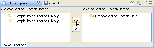
If you create a shared function library, the library can be added to other models or removed from current model by selecting the Shared Functions -folder and using the properties view.
External Functions
Modelica allows you to use external functions that are programmed using C language. To use this feature, you need to have the Sysdyn version with OpenModelica included and OpenModelica set as the solver in the Preferences (Window → Preferences → Solver). The installation package with OpenModelica has also MinGW C compiler included that allows to build object files from C source code.
Below is a simple example of using a function that returns the sum of two arguments.
 double exampleCFunction(double x, double y)
 {
   double res;
   res = x + y;
   return res;
 }
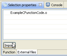
You need to create an Object file (.o) of your code, import it to a function and define the function to use the library and function that you created. If you don’t have a C-compiler, you can use the one provided by the Simantics installation (e.g. simantics_home/plugins/org.simantics.openmodelica.win32_x/MinGW/bin/mingw32_gcc.exe -g -O -c ExampleCFunctionCode.c).
You can use the external function like any other function in your variables. Using equation ExampleExternalFunction(Stock1, 10) in an auxiliary variable (Auxiliary2) gives the following result.
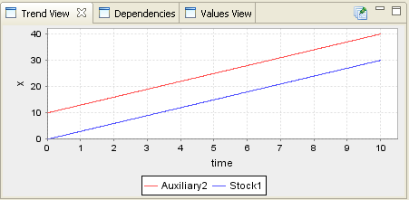
In addition to .o -files, you can import .c and .h files. By including these to the function, the source code can be reviewed and later by you or others that use the function.
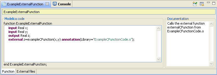
Small external C function can also be written directly to the function code in Simantics Sysdyn:
 function ExampleExternalFunction
 input Real x;
 input Real y;
 output Real z;
 external "C" z=exampleCFunction(x,y) annotation(Include="
 double exampleCFunction(double x, double y)
 {
   double res;
   res = x + y;
   return res;
 }");
 end ExampleExternalFunction;
Modelica Functions
Modelica has built-in functions that can be used anywhere and are not visible in function libraries. This section covers a large number of those functions. For functions related to array variables, see see Built-in functions for arrays.
| Function | Description |
|---|---|
| abs(x) | Returns the absolute value of x. Expanded into "(if x >= 0 then x else -x)". |
| acos(x) | Inverse cosine. |
| asin(x) | Inverse sine. |
| atan(x) | Inverse tangent. |
| atan2(x1,x2) | four quadrant inverse tangent. |
| cat(n,A,B,...) | General concatenation function that concatenates arrays A,B,... along the nth dimension. |
| ceil(x) | Returns the smallest integer not less than x, the closest integer above x. |
| cos(x) | Cosine. |
| cosh(x) | Hyperbolic cosine. |
| cross(x,y) | Returns the 3-vector cross product of the 3-vectors x and y. |
| delay(expr, delayTime) | Returns the value of expr at the time time-delayTime. The value of expr is returned when time <= time.start + delayTime. |
| der(x) | Time derivative of x. X must be have continuous-time variability. |
| div(x, y) | Returns the algebraic quotient x/y with any fractional part discarded. E.g. div(10,3) = 3. |
| edge(b) | Returns true when the value of the Boolean expression b changes. Expanded into (b and not pre(b)). |
| exp(x) | Exponential, base e. |
| floor(x) | Returns the largest integer not greater than x, the closest integer below x. |
| initial() | Returns true at the beginning of the simulation. |
| integer(x) | Returns the largest integer not greater than x as an integer. |
| log(x) | Natural logarithm. (base e, x > 0) |
| log10(x) | Base 10 logarithm. (x > 0) |
| mod(x, y) | Returns the integer modulus of x/y: mod(x,y) = x - floor(x/y) * y. |
| noEvent(expr) | noEvent around an expression causes the expression to NOT generate event. Important: If you want a condition to be checked only on time steps, use noEvent. (e.g. if noEvent(value >= 1) then ... else ...) |
| pre(x) | Returns the preceding value of y from time event that has occurred before current time. |
| rem(x, y) | Returns the integer remainder of x/y: rem(x,y) = x - div(x,y) * y. |
| sample(start, interval) | Returns true and triggers time events at times start + i * interval (i=0,1,...). |
| sign(x) | Returns -1 if x is negative, 1 if x is positive. Expanded into "(if x > 0 then 1 else if x < 0 then -1 else 0)". |
| sin(x) | Sine. |
| sinh(x) | Hyperbolic sine. |
| sqrt(x) | Square root of x. The value of x must be greater or equal to 0 or an assertion error occurs. |
| tan(x) | Tangent. |
| tanh(x) | Hyperbolic tangent. |
| terminal() | Returns true at the end of a successful simulation. |
Spreadsheets
Spreadsheets allow storing and maintaining values in a familiar format. The current spreadsheet implementation is experimental and does not provide much functionality.
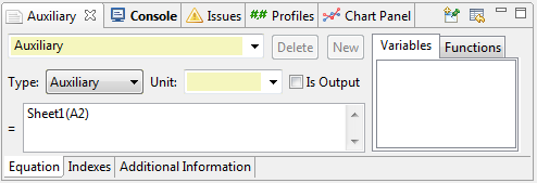
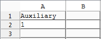
Variable Values
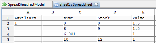
Spreadsheets are an easy way to import and manage parameter values. Sheet shells can be referenced to in models with the syntax SheetName(CellReference). Below is an example of getting a value for Auxiliary. The text "Auxiliary" is not necessary in the spreadsheet, but it helps maintaining the sheet.
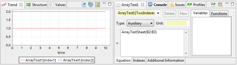
You can also refer to sheets with array variables. Reference is simple with one and two dimensional array variables. Below is an example of a sheet with values for two different variables. The names of the indices are not mandatory, but help reading and maintaining the sheet.
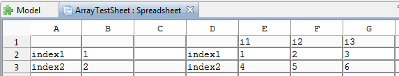
Reference to a sheet range creates an array variable.
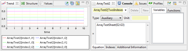
ArrayTest2 has two dimensions. Reference to a larger range creates a two-dimensional variable. By default, the indices are ordered as in this example. However, if you wish to present the indices in a different order in the spreadsheet, you can transpose the sheet reference (e.g. transpose(ArrayTestSheet(E2:G3)))
History Data
Spreadsheets can be used to store and display external history data e.g. from some statistics. The history data should be arranged as columns or rows and include a time variable. Reference variables need to be given the exactly same name as their counterparts in model.
History data is used by creating a History dataset to an experiment. The dataset is activated and deactivated in charts by double-clicking the dataset. History data reference is set in the properties of the history dataset.
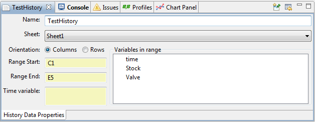
| History data properties | - |
|---|---|
| Name | Name of the history dataset |
| Sheet | Combo box for selecting a sheet where the history data is located |
| Orientation | Columns or rows. How the data is arranged in the sheet. |
| Range start | The upper-left corner cell of the history data range |
| Range end | The lower-right corner cell of the history data range |
| Time variable | The name of the time variable in the history data, if it is different than "time" |
| Variables in range | This text field displays the found variables in the given sheet and range |
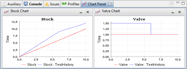
If the history dataset is activated, history data is displayed whenever it is available for a variable that is displayed in a chart.
Vensim Model Import
The tool also has a limited support for importing system dynamics models created with the simulation and modelling tool Vensim. This functionality is used similarly to the regular model import, so by right-clicking the browser and selecting "Import" → "Vensim Model (.mdl)".
The import process has several known limitations:
The Vensim model must be in the .mdl file format, the other Vensim file formats are proprietary and thus not supported.
Only variables and connections are imported.
Many advanced Vensim features, such as input and output objects (e.g. graphs and parameter value editors) and other diagram customizations, are not supported.
Variable value range data is not always imported correctly.
Subscripts are automatically converted to enumerations which may sometimes lead into problems as the constructions are not exactly equivalent.
Dimensionless units are currently not converted correctly (in Simantics System Dynamics, dimensionless should be indicated with a constant).
Non-shadow duplicate variables are sometimes very problematic and may be imported incorrectly, shadow variables should work fine.
Only a limited subset of Vensim functions is currently implemented in Simantics System Dynamics, so some equations might require additional work before they can be evaluated correctly.
Sample Models and Molecules
There are some sample models located in the sampleModels folder found in the installation folder. The sample models can be imported by right-clicking on the model browser and select Import→Model.
Further Reading
Tutorial: Basic System Dynamics Modelling
System dynamics modelling in Simantics is a free modelling tool that is included into the basic installation. This tutorial introduces the basic features of the system dynamics modelling tool.
Tutorial: Advanced System Dynamics Modelling
This tutorial introduces the more advanced features of the system dynamics modelling tool: Modules and Operating interfaces